In this guide
A data acquisition (DAQ) system measures physical conditions—force, vibration, pressure, temperature, or displacement—through conditioned analog channels and converts them into time-aligned digital samples. Every measurement chain combines three core stages: a transducer, analog signal conditioning, and an analog-to-digital converter (ADC) paced by a hardware clock. On packaging and weighing equipment, a dedicated DAQ is warranted whenever transient impacts outrun a PLC scan cycle, when conveyor resonances must be separated from true mass signals, or when load cells, accelerometers, and encoders must be correlated on a single timeline.
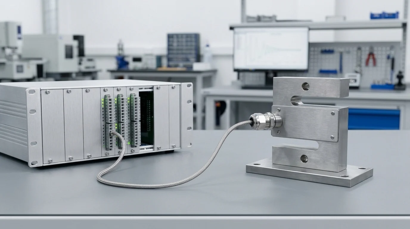
What is a data acquisition system?
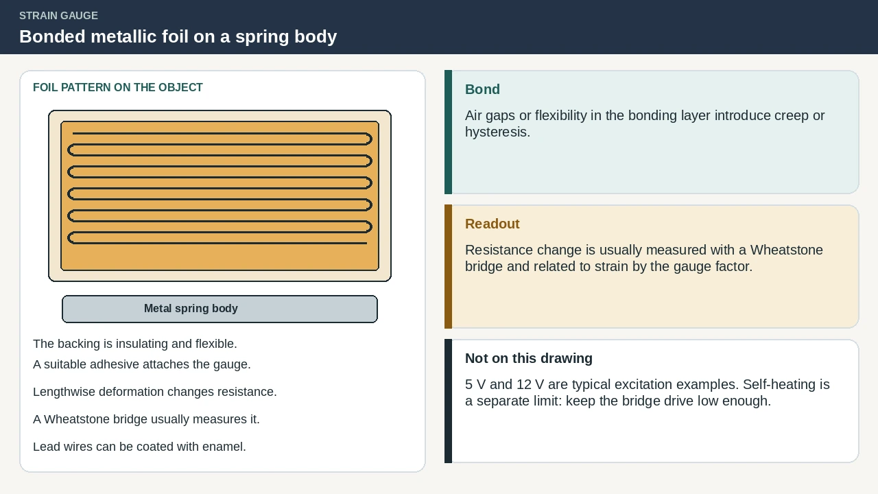
Data acquisition starts at the transducer, where a physical variable is converted into an electrical response—resistance change in a foil strain gauge or RTD, microvolt potential in a thermocouple, or charge in a piezoelectric accelerometer. Complete DAQ hardware pairs sensor-specific conditioning cards with high-precision ADCs, hardware timers, buffer RAM, and a bus or network interface to host acquisition software.
Signal conditioning prepares the raw transducer output so the converter operates near full scale without distortion or out-of-band noise. Depending on the sensor type, this front end provides regulated voltage or current excitation, bridge completion, high-impedance differential amplification, input overvoltage protection, galvanic isolation, linearization, and analog anti-aliasing filtration. Because an unamplified strain-gauge load cell outputs only a few millivolts across a several-volt common-mode pedestal, wiring it straight into a general-purpose 0–10 V ADC forfeits almost the entire dynamic range of the converter.
Inside a DAQ board or chassis, an onboard controller or FPGA coordinates trigger detection, hardware sample clocks, multiplexer switching, and direct memory transfers so sampling proceeds with deterministic timing jitter. Embedded microcontroller boards suit fixed-function, high-volume designs where control firmware never changes in the field, while industrial PLCs prioritize ruggedized sequential machine control. Neither a microcontroller input pin nor a PLC program scan replaces the analog conditioning stage ahead of the ADC.
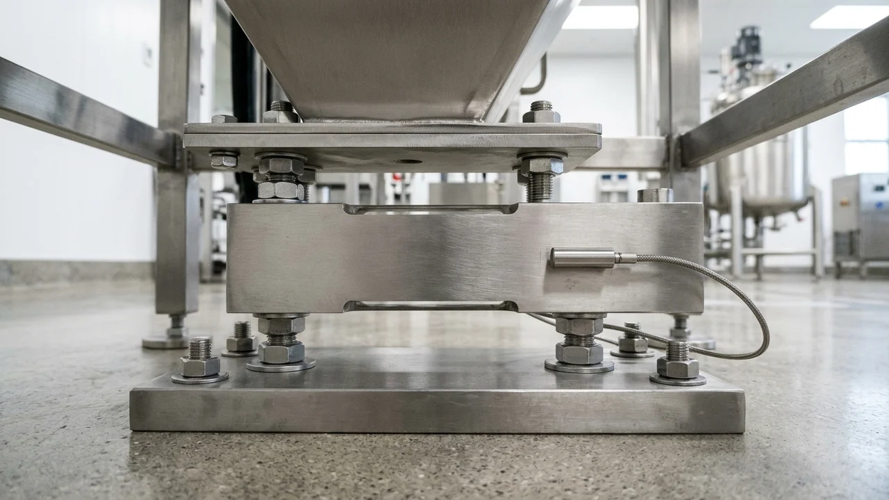
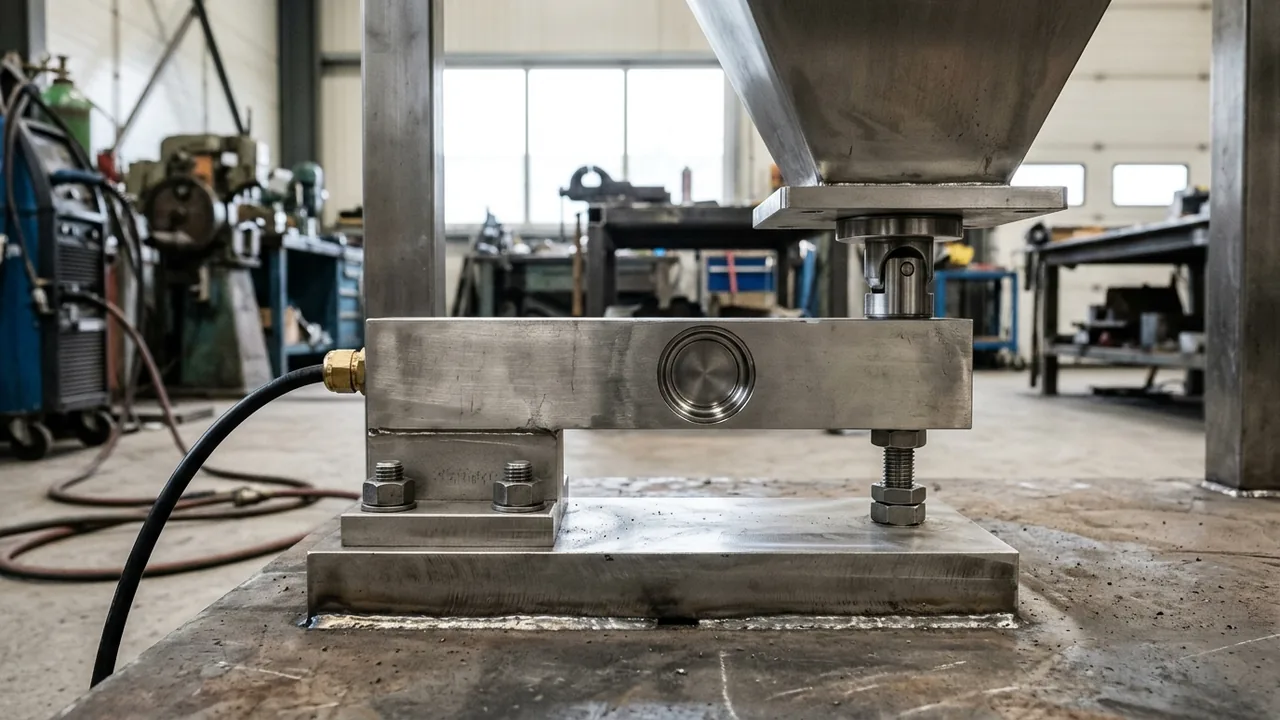
For the mechanical-to-electrical path inside packaging scales and hoppers, see the load cells and controls hub and the broader measurement guides on the home page.
Where do excitation and the anti-alias filter sit?
On a strain-gauge weighing channel, elastic deflection changes gauge resistance inside a four-arm Wheatstone bridge energized across one diagonal and read differentially across the other. A balanced bridge of matched resistors produces zero differential voltage, and uniform temperature drift across all four arms cancels to first order. When applied load unbalances the arms, an instrumentation amplifier—or the integrated low-noise programmable-gain amplifier (PGA) of a bridge ADC—reads that small differential voltage with high input impedance, low DC offset drift, and high common-mode rejection.
Excitation stability directly governs scale accuracy unless the converter measures ratiometrically. Industrial strain-gauge load cells typically specify 5 V to 10 V DC excitation (with AC or switched-DC excitation reserved for ultra-low-drift laboratory or high-EMI environments to cancel thermoelectric offsets) and tie the ADC reference pins directly to the excitation or six-wire sense lines so supply drift cancels out. Where motor drives, welding currents, or distant ground potentials threaten the measurement cabinet, galvanic isolation breaks the conductive path between the sensor side and the acquisition backplane.
Ahead of the sampler sits an analog anti-aliasing low-pass filter that restricts signal bandwidth to satisfy the Nyquist–Shannon sampling theorem, followed in successive-approximation (SAR) architectures by a sample-and-hold capacitor that freezes input voltage during conversion. As NIST’s DFT guidance notes, a practical anti-aliasing filter balances flat passband magnitude, linear phase (constant group delay) across the band of interest, and steep stopband attenuation before half the sampling rate:
- Bessel response: Preserves linear phase and step waveform shape with minimal overshoot, making it preferable when transient peak force or time-domain alignment across channels matters.
- Butterworth response: Delivers a maximally flat passband amplitude for spectral energy measurements, at the cost of nonlinear phase shift below the corner frequency.
- Sharp-cutoff (elliptic or high-order Chebyshev) filters: Maximize frequency-domain selectivity near Nyquist, though steep analog walls introduce step ringing that corrupts short weighing windows.
Oversampling eases all three compromises: raising the ADC sampling rate pushes the Nyquist limit upward so a gentler, higher-cutoff analog RC or active filter can suppress aliases without phase-distorting low-frequency force signals. Gain staging must also prevent amplifier saturation after the filter, because clipping generates harmonic distortion above the filter passband that subsequently folds into the digitized record.
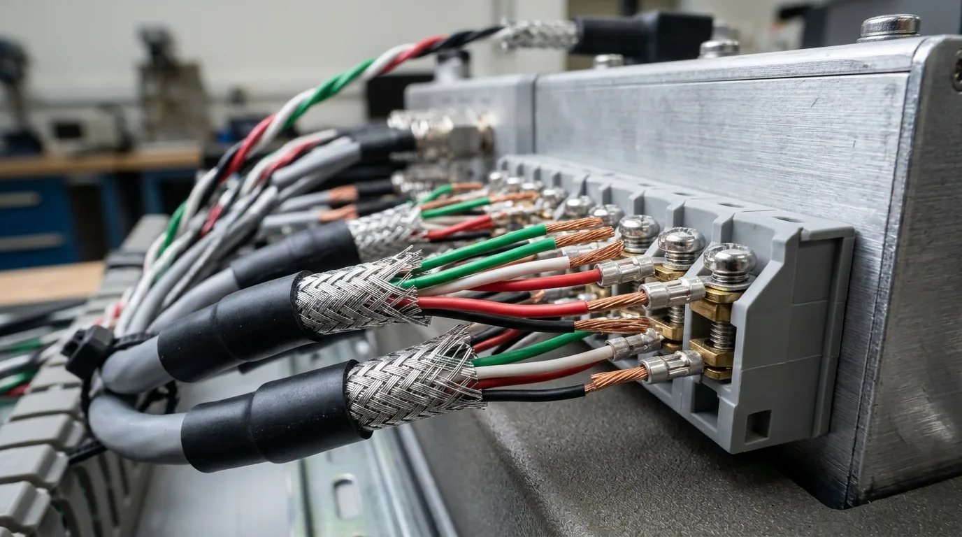
Cable voltage drop and sense-lead wiring for that front end are covered in the Wheatstone bridge wiring guide.
Why does a missing low-pass fold vibration into the samples?
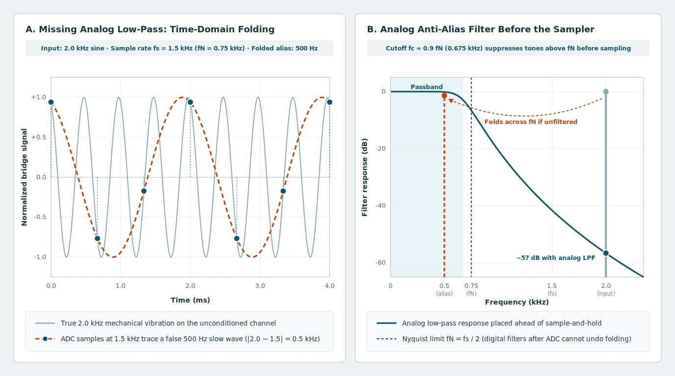
To capture a bandlimited signal without aliasing, the sampling rate (fs) must exceed twice the highest frequency component present at the converter input—meaning every analog component must stay below the Nyquist frequency (fN = fs / 2), half the sampling rate. When frequencies above the Nyquist frequency (half the sampling rate) reach the sampler, each individual voltage sample can still be quantized accurately, yet the discrete points trace a false lower-frequency waveform that cannot be separated from genuine low-frequency load changes after conversion. Digital filtering inside software or a PLC cannot undo this folding because the alias already occupies the passband of the recorded data.
A standard textbook benchmark illustrates the arithmetic: sampling an unfiltered 2.0 kHz sine wave at 1.5 kHz (fN = 0.75 kHz) folds the tone to |2.0 − 1.5| = 0.5 kHz, producing an apparent 500 Hz oscillation in the sample stream. Because real analog filters roll off gradually rather than at a vertical brick wall, instrumentation designs set the usable passband cutoff below fN—for example, Colorado State University’s DSP laboratory notes place a practical analog cutoff near 90 percent of the Nyquist frequency (3.6 kHz for an 8 kHz sample rate), reserving the remaining transition band for stopband attenuation.
Weighing and checkweigher front ends solve this problem primarily with 24-bit delta-sigma (ΣΔ) ADCs. Because a delta-sigma modulator oversamples the bridge at hundreds of kilohertz to several megahertz before digital decimation, a simple differential RC low-pass filter at the input pins suffices to block RF interference and modulator-clock aliases, while internal sinc (sinc³/sinc⁴) or FIR digital filters establish the sharp measurement cutoff:
- Static platform and bench scales: Commonly output at 5 to 20 samples per second (SPS) with effective low-pass cutoffs of 1 to 5 Hz and simultaneous 50/60 Hz mains notches to maximize noise-free resolution.
- Dynamic checkweighers: With package weigh-platform dwell times often between 50 and 200 ms, weight transmitters typically run ADC output data rates from 100 Hz to 1 kHz (and up to 4.8 kHz on fast multi-channel transmitters), placing the digital low-pass cutoff below dominant roller, belt-seam, and frame vibration frequencies—typically 5 to 25 Hz, tuned so the step response still settles completely inside the active checkweigher zone window.
- Modal and impact test stands: When diagnosing conveyor frame resonances, bearing defects, or drop-impact shocks with SAR DAQ cards, sample at 5 to 50 kHz per channel behind matched hardware anti-aliasing filters so structural harmonics never fold into the force trace.
When is a dedicated DAQ required?
Choosing between a PC- or network-tethered DAQ, a standalone data logger, and a PLC input module comes down to sample clock rate, channel synchronization, and where the measurement record is consumed.
Standalone data loggers combine local memory, low-power conditioning, and unattended autonomy for multi-day or continuous 24-hour monitoring—such as tracking ambient temperature, supply voltage stability, or thermal zero drift around a load-cell installation. Sample rates around 1 Hz are routine for loggers and well matched to slowly varying thermal signals, whereas dynamic force and vibration capture starts two to four orders of magnitude faster.
An industrial PLC executes a deterministic cyclic scan: read inputs, solve control logic, and update outputs. Scan times commonly span several milliseconds to tens of milliseconds, with additional latency and jitter across remote fieldbus racks. Standard PLC analog inputs (0–10 V or 4–20 mA) work reliably when an external weight transmitter has already conditioned, filtered, and scaled the load cell—trade-offs detailed in the load cell amplifier and fieldbus guide. Slow integrating ADCs likewise suit steady-state scale displays and thermocouples. By contrast, high-speed shaft encoders require dedicated PLC hardware counter modules rather than scan-polled discrete inputs, and multi-sensor transient waveform capture calls for a dedicated DAQ clocked independently of machine logic.
| Architecture | Timing & sample rate | Where data lives | Packaging & weighing role |
|---|---|---|---|
| Tethered or networked DAQ | Hardware sample clock; typically 100 Hz to 50+ kHz per channel | Host PC or chassis buffer RAM | Impact profiling, conveyor vibration diagnostics, and synchronized multi-sensor trials |
| Standalone data logger | Slow periodic clock; typically ≤ 1 Hz to 10 Hz | Non-volatile onboard memory | Unattended thermal drift, power quality, and environmental logging |
| PLC scan with fieldbus I/O | Cyclic scan (milliseconds to tens of ms) plus hardware counter cards | Controller registers via transmitter or remote I/O | Production line sequencing, fill cutoff control, and reject actuation |
How does a multiplexer change the sample clock?
Many multi-channel DAQ boards route several conditioned inputs through an analog multiplexer—a solid-state switch array—into a single shared ADC. Sharing one converter lowers hardware cost and board area, but divides the aggregate conversion rate across active channels: an 80 kS/s converter scanning 8 channels delivers 10 kS/s per channel, and visits those channels sequentially rather than at the exact same instant.
Sequential scanning introduces inter-channel phase skew. Comparing a load-cell transient on channel 1 directly against an accelerometer on channel 8 without accounting for multiplex delay creates an artificial time lag at higher frequencies. Where true phase alignment is required—such as subtracting frame acceleration from a dynamic weighcell signal or computing three-axis force vectors—the front end must either place simultaneous sample-and-hold amplifiers ahead of the multiplexer on a common pacing clock, or dedicate an independent synchronized ADC per channel.
How are mixed sensor channels kept in step?
Commissioning a high-speed weighing or filling machine frequently combines millivolt Wheatstone bridges, 4–20 mA pressure transmitters, thermocouples or RTDs, accelerometers, and rotary shaft encoders in one test setup. Keeping those heterogeneous signals aligned requires matching each analog front end to its transducer before locking every channel to a shared sample or timestamp clock.
Rose-Hulman’s signal-conditioning benchmark highlights why strain-gauge channels demand dedicated front-end gain rather than direct connection to volt-level inputs: given a 120 Ω bridge, metallic foil gage factor GF ≈ 2, strain ε = 0.001 (1,000 µε), and 10 V excitation, a single active quarter-bridge arm outputs Vout ≈ Vex × GF × ε / 4 = 5 mV, while a four-active-arm push-pull bridge outputs Vout = Vex × GF × ε = 20 mV. Across commercial load cells rated at 2 mV/V, full-scale output is 10 mV at 5 V excitation or 20 mV at 10 V excitation, and partial-load dynamic swings routinely sit around ±2 mV (the millivolt range noted in Virginia Tech’s instrumentation manual, rather than volts or microvolts).
To bring that ±2 mV to 20 mV bridge signal onto the same timeline as volt-level and digital sensors:
- Bridge channels: Apply ratiometric 5–10 V excitation and 64× to 500× low-noise differential gain (depending on whether the ADC full scale is ±20 mV internal PGA range or ±5 V / ±10 V modular DAQ input), followed by matched anti-alias filtering.
- Current-loop and voltage transmitters: Convert 4–20 mA across precision shunt resistors and match filter group delay if transients are compared directly against raw bridge waveforms.
- Encoder and photo-eye timing: Route quadrature conveyor encoders and package-entry photo-eyes into hardware counter-timer channels latched on the same sample clock so belt position is recorded alongside every force sample.
Selection checklist for the channel and the clock
Use this specification checklist when qualifying a multi-channel force, vibration, or packaging measurement system:
- Channel mix and full-scale spans: List each bridge (mV/V sensitivity), 4–20 mA loop, temperature sensor, accelerometer, and encoder channel.
- Excitation, sense, and isolation: Specify regulated 5 V or 10 V ratiometric excitation with six-wire sense compensation where cables run long, plus channel-to-channel or bank isolation near VFD motor wiring.
- Signal and disturbance bandwidth: Identify both the fastest weighing step or impact to preserve and the dominant roller, drive, or structural vibration frequencies above it.
- Anti-aliasing and ADC architecture: Pair SAR channels with hardware Bessel or Butterworth low-pass filters below
0.5 × fs(typically≤ 0.45 × fs), or select 24-bit delta-sigma bridge channels whose digital filter settles within the available weigh dwell time. - Cross-channel synchronization: Require simultaneous sample-and-hold or per-channel synchronized ADCs whenever force, acceleration, and encoder position are correlated in time.
- System role: Assign continuous control and reject timing to the PLC or weight controller, slow unattended monitoring to a logger, and high-rate waveform diagnostics to the dedicated DAQ.